28. Loss of the Neural Network
28.1. Error Surface&等高线
- 在Hilton和Andrew的课中,多次提及这个概念。
- 在图中,可以看出weights的运行轨迹。
- 下图就是一个linear neuron的error surface的垂直截面图和水平截面图,水平轴是each weight,垂直轴是error。
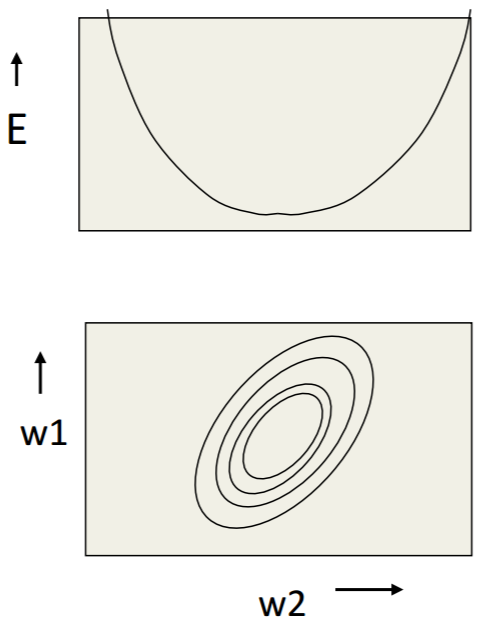
从上图可得:
- 梯度下降法的作用就是不断调整参数,使得模型的误差由“碗沿”降到“碗底”,参数由椭圆外部移动到椭圆的中心附近。
- weights每一个分量的变化(gradient descent)的矢量和就是cost function收敛的方向
28.2. Loss of each sample
只有在“training”阶段才会用 “loss” 这个词,而在”validation”和”test”阶段,则会用“true or false of each sample”等概念。
不同的场景,有不同的方式来计算”the loss of each sample”,可以参见本章下面的小节。 一般而言,只有先写出”loss of each sample”的计算公式,才能写出”loss the network”的计算公式。
28.3. Loss of the network
只有在”training”阶段,才会用”loss of the network”这个概念,而在”validation”和”test”阶段,会用“网络精度”或者“网络准确率”等来量化”performance of the network”。
其实,”loss of the network”表述不准确,应该称为”loss of the batch”或者”learning target”,并且要和”loss of each sample”的含义进行区分。
对于mini/full batch learning method而言, “learning target” 被定义为“batch中每个sample的loss的均值”,见《tf实战》p90函数loss()中使用了tf.reduce_mean()
28.3.1. Implement in TF
如果网络loss的定义中是几个项相加,TF采用的方法是先定义各个子项,然后加起来。例如,对卷积网络中全链接层的weight进行regularization时(除去卷积层和softmax层的weight),是如何处理的,《tf实战》5.2
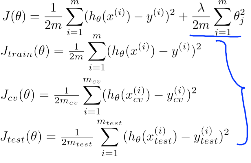
28.4. 回归场景的loss
IN regression problem, we employ the Euclidean(欧几里德) loss for each sample.
(from Andrew Ng Week6)
28.4.1. 在tf中的实现
1 2 3 4 | #shape of bbox_pred is [batch,4]
square_error = tf.square(bbox_pred-bbox_target)
#@shape(square_error)=[batch_size]
square_error = tf.reduce_sum(square_error,axis=1)
|
28.6. 多分类场景的loss
使用softmax作为神经网络最后一层输出,在testing set上计算的是“准确率”,而非loss。
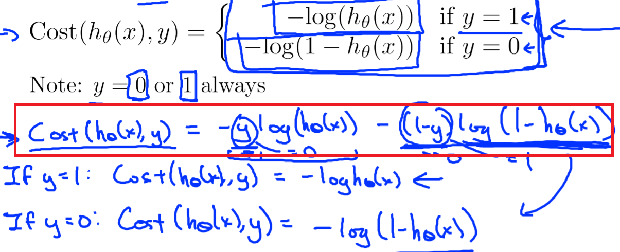
28.6.1. loss when trainning
一个softmax group包括多个neurons,它们作为一个整体作为output layer时的loss称为“Cross Entropy(互熵)”。 FOR EACH SAMPLE, the loss is:
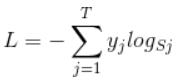
首先L是损失。Sj是softmax的输出向量S的第j个值,前面已经介绍过了,表示的是这个样本属于第j个类别的概率。yj前面有个求和符号,j的范围也是1到类别数T,因此y是一个1*T的向量,里面的T个值,而且只有1个值是1,其他T-1个值都是0。那么哪个位置的值是1呢?答案是真实标签对应的位置的那个值是1,其他都是0。所以这个公式其实有一个更简单的形式:
当然此时要限定j是指向当前样本的真实标签。
来举个例子吧。假设一个5分类问题,然后一个样本I的标签y=[0,0,0,1,0],也就是说样本I的真实标签是4,假设模型预测的结果概率(softmax的输出)p=[0.2,0.3,0.4,0.6,0.5],可以看出这个预测是对的,那么对应的损失L=-log(0.6),也就是当这个样本经过这样的网络参数产生这样的预测p时,它的损失是-log(0.6)。那么假设p=[0.2,0.3,0.4,0.1,0.5],这个预测结果就很离谱了,因为真实标签是4,而你觉得这个样本是4的概率只有0.1(远不如其他概率高,如果是在测试阶段,那么模型就会预测该样本属于类别5),对应损失L=-log(0.1)。那么假设p=[0.2,0.3,0.4,0.3,0.5],这个预测结果虽然也错了,但是没有前面那个那么离谱,对应的损失L=-log(0.3)。我们知道log函数在输入小于1的时候是个负数,而且log函数是递增函数,所以-log(0.6) < -log(0.3) < -log(0.1)。简单讲就是你预测错比预测对的损失要大,预测错得离谱比预测错得轻微的损失要大。
28.6.2. loss when testing
注意:使用softmax作为神经网络最后一层输出,在testing set上计算的是“准确率”,而非loss。
《tf实战》p91 tf.nn.in_top_k()
28.7. OHEM(Online Hard Sample Mining)
MTCNN给出了OHEM的解释: In particular, in each mini-batch, we sort the loss computed in the forward propagation phase from all samples and select the top 70% of them as hard samples. Then we only compute the gradient from the hard samples in the backward propagation phase. That means we ignore the easy samples that are less helpful to strengthen the detector while training.
以多分类场景为例,在“训练阶段”,计算softmax层的”cross entropy loss”时,OHEM其实只是“多做了一步计算”而已。
1 2 3 4 5 6 7 | #这段代码改编自《tf实战》p90
#mini-batch learning method
#shape of cross_entropy is [batch_size]
cross_entropy = tf.nn.sparse_softmax_cross_entropy_with_logits()
#OHEM其实就是多加了如下的这一步计算而已
cross_entropy = tf.nn.top_k(cross_entropy, k)
cross_entropy_mean = tf.reduce_mean(cross_entropy)
|